
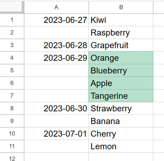
I’m using Google Sheets. In column A there are dates at irregular intervals. In column B there are names of fruit. I’d like to add some conditional formatting depending on the date corresponding to the fruit or, if the fruit doesn’t have one, the lowest one above it (you may assume there will always be a date in cell A1). The effect is that a date affects the fruit next to it and all consecutive fruits up until the next date given.
I imagine I’d have to add a lookup by criterion NOT(ISBLANK()) to the conditional formatting custom formula. Is there a function that could do that? Is there some other way I can achieve the desired result?
Example image:
You must log in or register to comment.